Searching
Data Structure
Searching
Read Map
Static Search Table
Sequential Search
Binary Search
Indexing Search
Binary Search Trees (Dynamic Search Table)
Binary search tree
AVL tree
B-Tree
Hash Table
What is hashing
Hash Function
Collision Resolution
Closed Hashing
Open Hashing
Analysis of Hashing
Search Table
Definition
A set of the same type of data elements
Key
The value of data item in the data element. It is used to identify the data elements
Primary Key and Second Key
Searching
Based on the search value of key find out the element whose key value is same as search value
It returns the position of the element located in
Operations on searching table
-
Search a given element in the search table
-
Get attributes of a given element
-
Insert an element into the search table
-
Delete an element from the search table
Static Search Table
Only do search on the search table
Dynamic Search Table
Need do search and insertion and deletion on the search table
Basic concepts
Given: Distinct keys $k_1 , k_2 , …, k_n$ and collection T of n records of the form $((k_1 , I_1 ), (k_2 , I_2 ), …, (k_n , I_n ))\newline$
where $I_j$ is the information associated with key $k_j\ for\ 1 \leq j \leq n\newline$
Search Problem
For key value K, locate the record $(k_j , I_j)$ in T such that $k_j = K\newline$
Search
Searching is a systematic method for locating the $record(s)$ with key value $k_j = K\newline$
Successful vs Unsuccessful
A successful search is one in which a record with key $k_j = K$ is found
An unsuccessful search is one in which no record with $k_j = K$ is found (and presumably no such record exists)
We often ask how many times one key is compared with another during a search.
This gives us a good measure of the total amount of work that the algorithm will do
Approaches to Search
-
Sequential and list methods (lists, tables, arrays).
-
Tree indexing methods
-
Direct access by key value (hashing)
Static Search Table
Sequential Search
|
|
General Idea
Begin at one end of the list and scan down it until the desired key is found or the end is reached
A successful search returns the position of the record
An unsuccessful search returns 0
|
|
Analysis
To analyze the behavior of an algorithm that makes comparisons of keys
we shall use the count of these key comparisons as our measure of the work done
Average Search Length(ASL)
$$ ASL=P_1C_1+P_2C_2+…+P_nC_n=\sum_{i=1}^nP_iC_i\newline $$ $Where\ P_i\ is\ probability(frequency)\ of\ search\ i^{th}\ record\newline$ $and\ C_i\ is\ the\ count\ of\ key\ comparisons\ when\ search\ it\newline$
$for\ sequential\ search$ $$ \begin{align} &success\rightarrow\newline &best\ case:\ 1\ comparison\newline &worst\ case:n\ comparisons\newline &average\ case:ASL_{sq}=\sum^n_{i=1}P_iC_i=\sum^n_{i=1}\frac {1}{n}(n-i+1)=\frac {n+1}{2}\newline\newline &unsuccessful\ search:\rightarrow n+1\ comparisons\newline \end{align} $$
Binary Search
Ordered List
An ordered list is a list in which each entry contains a key, such that the keys are in order
That is, if entry $i$ comes before entry $j$ in the list, then the key of entry $i$ is less than or equal to the key of entry $j$ .
Idea
In searching an ordered list, first compare the target to the key in the center of the list.
If it is smaller, restrict the search to the left half. otherwise restrict the search to the right half
and repeat. In this way, at each step we reduce the length of the list to be searched by half
Initialization: Set Low=1 and High= Length of List
Repeat the following $$ \begin{align} &If\ Low > High, Return\ 0\ to\ indicate\ Item\ not\ found\newline &mid=\frac{low+high}{2}\newline &if\ (K<ST[mid])\rightarrow high=mid - 1\newline &else\ if\ (K>ST[mid])\rightarrow low = mid + 1\newline &else\ return\ mid\ as\ location\ of\ the\ target\newline \end{align} $$
code
URL $\rightarrow$ https://zhuanlan.zhihu.com/p/565438258
$Three\ editions:\ 《Data\ Structure》\ from\ Tsinghua\ University\ -\ Deng\ Junhui\newline$
|
|
|
|
|
|
Analysis
$$ \begin{align} &T(n)=T(\frac{n}{2})+O(1)\newline &T(n)=T(\frac{n}{2})+O(1)=T(\frac{n}{4})+O(2)=T(\frac{n}{8})+O(3)=…=O(\log n)\newline \end{align} $$
Decision Tree
definition
The decision tree (also called comparison tree or search tree) of an algorithm is obtained by tracing the action of binary search algorithm, representing each comparison of keys by a node of the tree (which we draw as a circle)
Branches (lines) drawn down from the circle represent the possible outcomes of the comparison. When the algorithm terminates, we put either F (for failure) or the location where the target is found at the end of the appropriate branch, and draw as a square
Example
$$ array:[1, 2, 3, 4, 5, 6, 7, 8, 9, 10, 11]\newline $$
Analysis by decision tree
$$ \begin{align} &The\ best\ case:1\ comparison\newline &The\ worst\ case:the\ depth\ of\ a\ decision\ tree\ h\newline &The\ depth\ of\ a\ decision\ tree\rightarrow h=\lfloor \log_2n \rfloor+1\newline &O(\log_2 n)\newline &Average\ case(ASL): O(\log_2 n)\newline &ASL_{bn}=\sum^n_{i=1}P_iC_i=\frac {1}{n}[1 * 2^0 + 2 * 2^1 + 3 * 2^2 + … + h * 2^{h-1}]\newline &=\frac {n+1}{n}\log_2(n+1)-1 \approx \log_2(n+1)-1=O(log_2 n)\newline \end{align} $$
Indexing Search
Data Structure
Divided a search list R[n] into b sublist.
Each sublist may not be ordered by key, but the maximal key in the front sublist must be lower than the minimal key in the next successor list
An indexing table ID[b]. ID[i] stores the maximal key in i-th list. ID[b] is an ordered list
Idea
- Search in ID[b] to determine the possible sublist (Sequential search or binary search can be used)
- Search in R[n] (Only sequential search can be used)
Analysis
$ASL=ASL_{Index\ table}+ASL_{Sublist}\newline$
For search list of length n, it is divided into b sublist and the length of a sublist is $s = \frac {n}{b}\newline$
If using binary search in indexing table, the Average Search Length will be $log_2 (1 + \frac {n+1}{s})-1 + \frac {s + 1}{2}\newline$
If using sequential search in indexing table, the Average Search Length will be $\frac {b+1}{2} + \frac {s+1}{2} = \frac {s^2 + 2s + n}{2s}\newline$
For list of length 10000,
Sequential search: $ASL=\frac {n+1}{2}=5000\newline$
Indexing search (s=100):
$ASL= log_2 (b+1)-1+ \frac {S+1}{2} <57\newline$
$or ASL= \frac {b+1}{2} + \frac {S+1}{2} = 101\newline$
Binary search: $ASL=log_2 (n+1)-1 < 14\newline$
Summary and Comparison
| Sequential Search | Binary Search | Indexing Search | |
|---|---|---|---|
| ASL | Largest | Smallest | Middle |
| List Structure | Ordered Unordered | Ordered | Ordered indexing table |
| Storage Structure | Array or Linked List | Array | Array or Linked List |
Binary Search Trees (Dynamic search table)
Binary Search Tree
Definition
Binary Search Tree (BST) is a binary tree in which
-
Every element has a unique key.
-
The keys in a nonempty left subtree (right subtree) are smaller (larger) than the key in the root of subtree.
-
The left and right subtrees are also Binary Search Trees.
Note that this tree is ordered!
-
Each element to the left of the root is less than the root
-
Each element to the right of the root is greater than the root
Example
Search path
$Search\ path\ is\ a\ path\ from\ root\ to\ a\ node.\ The\ number\ of\ comparisons\ is\ the\ level\ of\ the\ node.\newline$
|
|
The searching efficiency is affected by the shape of Binary Search Tree
The worst case(one node per level, binary search degenerates to sequential search):$ASL=\frac {n+1}{2}\newline$
The best case (n nodes should have $\lfloor \log_2n\rfloor +1$ levels) :$ASL=\log_2 (n+1)-1\newline$
Insertion into BST
When search is not successful, the new data is inserted into BST
The new node must be a leaf of BST, and it is inserted into the position of searching fault
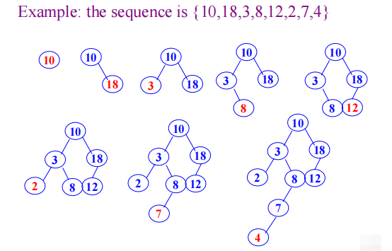
image1)Deletion from BST
-
The deleted node is a leaf node – delete node, reset link from parent to Null
-
The deleted node with 1 child – delete node, reset link from parent to point to child
-
The deleted node with 2 children
Let left subtree of P as left subtree of F;
Or Replace node with inorder predecessor (successor) S
Delete S (which has 0 or 1 child)
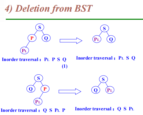
image1)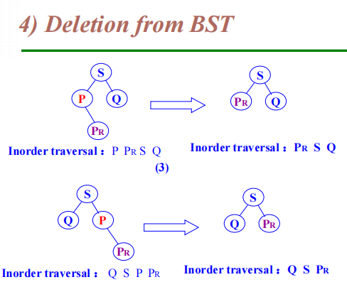
image2)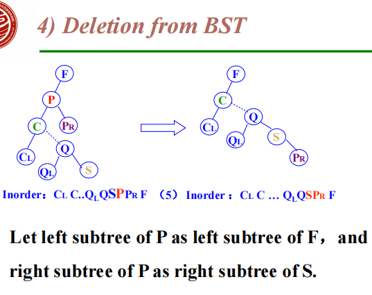
image3)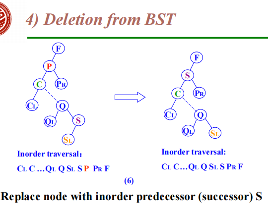
image4)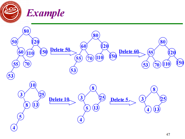
image5)
|
|
|
|
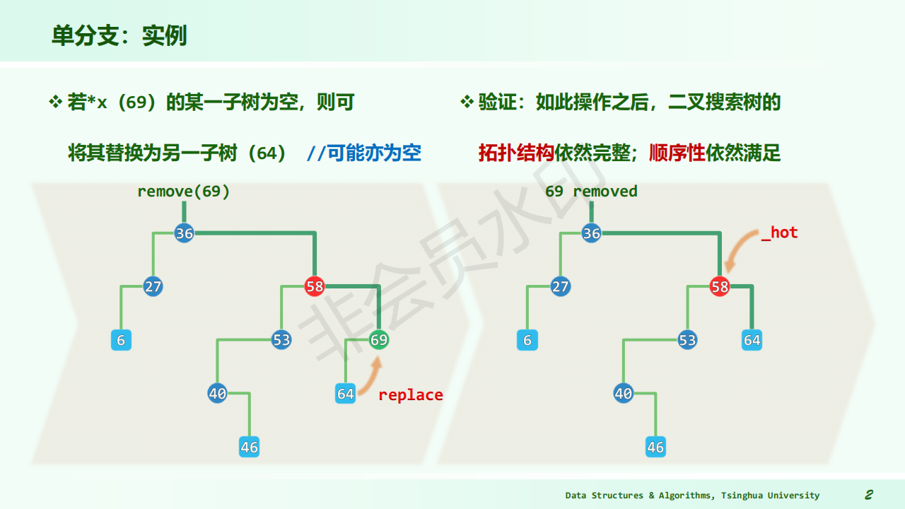
image1)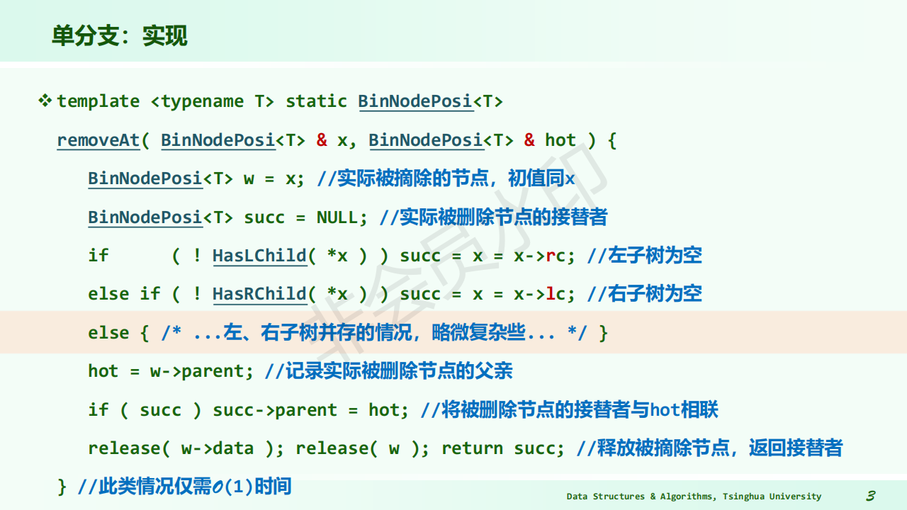
image2)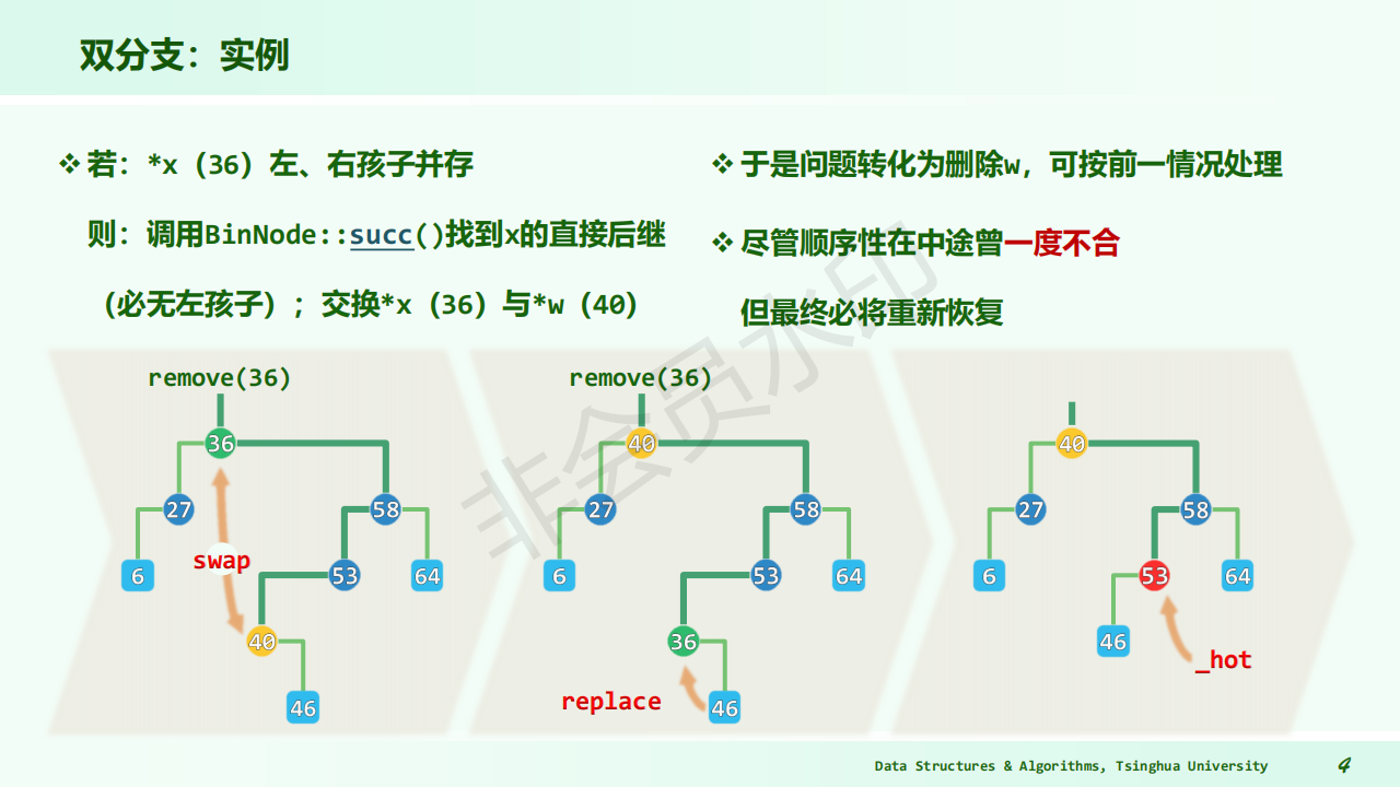
image3)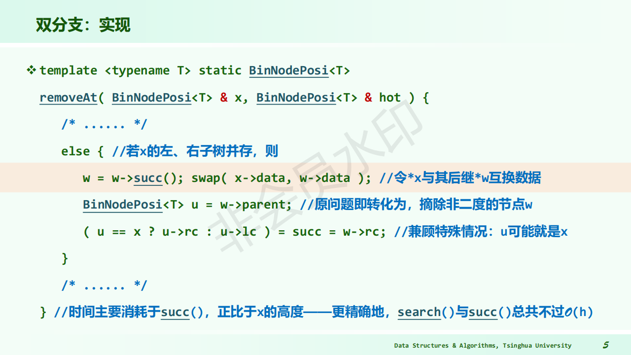
image4)AVL Tree
Tree Balancing
Binary Search Trees(BST) are designed for fast searching!
But the order of insertion into a BST determines the shape of the tree and hence the efficiency with which tree can be searched.
If it grows so that the tree is as “fat” as possible (fewest levels) then it can be searched most efficiently. If the tree grows “lopsided”, with many more items in one subtree than another, then the search efficiency will degrade.
For AVL(different in BST)
An AVL tree is a binary tree that is height balanced
$\rightarrow The\ difference\ in\ height\ between\ the\ left\ and\ right\ subtrees\ at\ any\ point\ in\ the\ tree\ is\ restricted\newline$
Balance Factor
Definition
The balance factor of node x to be the height of x’s left subtree minus the height of its right subtree.
$balFac(v)=height(lc(v))-height(rc(v))\newline$
An AVL tree is a BST in which the balance factor of each node is 0, -1, or 1
Example
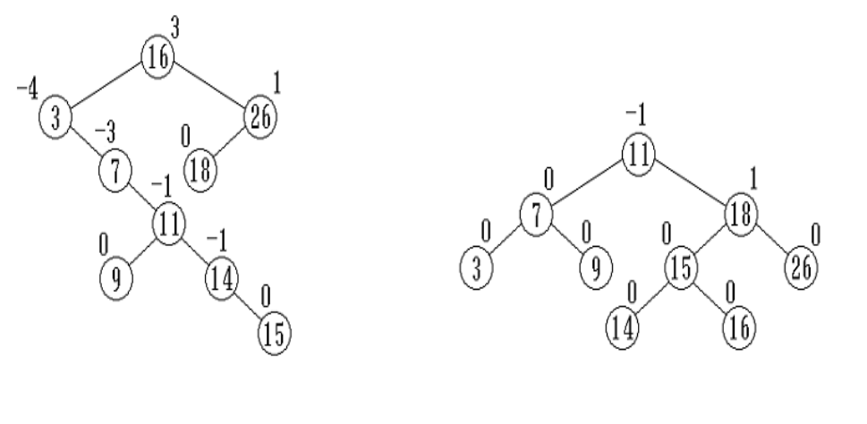
image1)insert
|
|
remove
|
|
refactoring->”3+4”
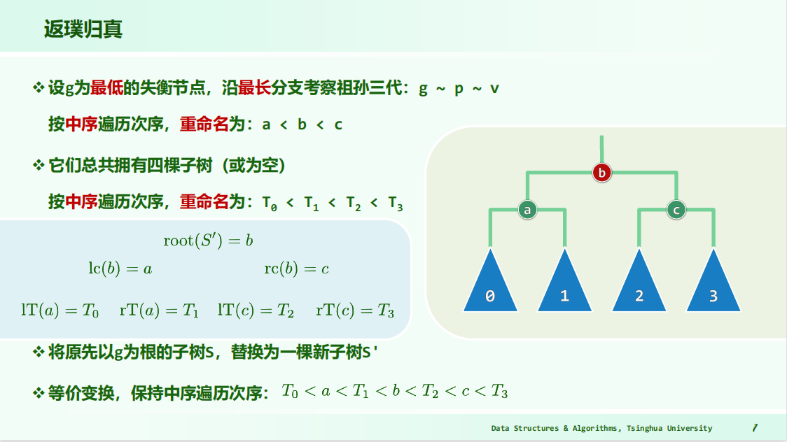
image1)
|
|
|
|
summary
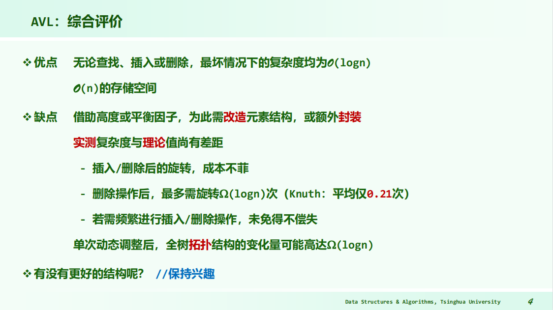
image1)B-Tree
Goals of Indexing
-
Store large files
-
Support multiple search keys
-
Support efficient insert, delete, and range queries
Difficulties when storing tree index on disk
- Tree must be balanced
- Each path from root to leaf should cover few disk pages
The B-Tree is now the standard file organization for applications requiring insertion, deletion, and key range searches
Definition
B-Tree of order m has these properties
-
The root is either a leaf or has at least two children
-
Each node, except for the root and the leaves, has between $\lceil \frac {m}{2} \rceil and\ m$ children
-
The number of Keys in each node(except for the root) is between $\lceil \frac {m}{2} \rceil-1\ and\ m-1\newline$
-
All leaves are at the same level in the tree, so the tree is always height balanced
Example
$B-Tree\ m=5\newline$
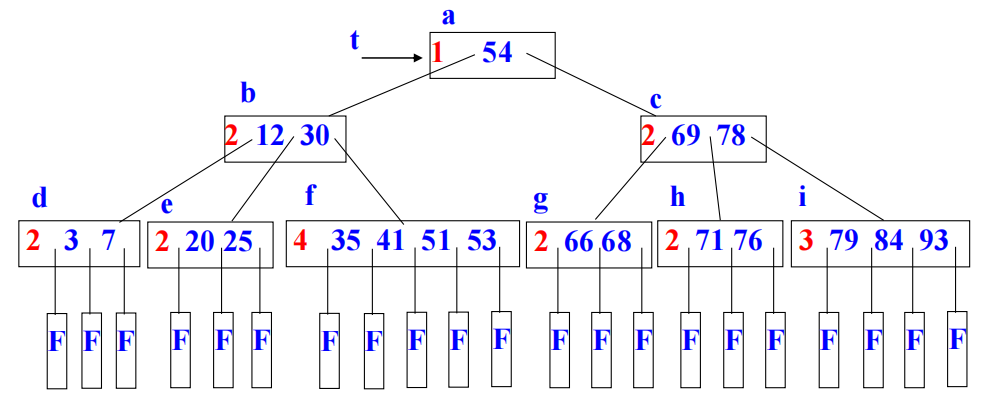
image1)Application
B-Tree node is usually selected to match the size of a disk block
B-Tree Search
Search in a B-Tree is similar with search in BST
-
Search keys in current node. If search key is found, then return record. If current node is a leaf node and key is not found, then report unsuccessful
-
Otherwise, follow the proper branch and repeat the process
B-Tree Insertion
To insert value X into a B-tree, there are 3 steps
-
using the SEARCH procedure for M-way trees (described above) find the leaf node to which X should be added
-
add X to this node in the appropriate place among the values already there. Being a leaf node there are no subtrees to worry about
-
if there are M-1 or fewer values in the node after adding X,then we are finished. If there are M values after adding X, we say the node has overflowed.
To repair this, we split the node into three parts:
-
Left: the first $\frac {M-1}{2}$ values
-
Middle: the middle value $(position\ 1+(\frac {M-1}{2}))\newline$
-
Right: the last $\frac {M-1}{2}$ values
-
B-Tree Deletion
-
How many values might there be in this combined node?
-
The parent node contributes 1 value
-
The node that underflowed contributes exactly $\frac {M-1}{2}-1$ values
-
The neighboring node contributes somewhere between $\frac {M-1}{2}\ and\ M-1$ values
case 1
Suppose that the neighboring node contains more than (M-1)/2 values. In this case, the total number of values in the combined node is strictly greater than 1 + ((M-1)/2 - 1) + ((M-1)/2)
case 2
Suppose, on the other hand, that the neighboring node contains exactly (M-1)/2 values. Then the total number of values in the combined node is 1 + ((M-1)/2 - 1) + ((M-1)/2) = (M-1)。
Hash Table
What is hashing
$Linear\ Search\ \rightarrow O(n)\newline$
$Binary\ Search\rightarrow O(\log_2n)\newline$
-
Both depend on comparisons of item sought and elements in container
-
Hash tables place data so that the location of an item is determined directly as a function of the item itself
-
With a good hash function, searching a hash table takes O(1) time. that is, it is a constant and does not depend on the number of items stored.
$Address(a_i)=Hash(a_i.key)\newline$
Here
$a_i\ is\ an\ element\newline$
$Address(a_i)\ stores\ the\ address\ of\ a_i\newline$
$a_i.key\ is\ the\ key\ of\ a_i\ element\newline$
General Idea
One problem with hash tables is collisions:
$\rightarrow $when more than one item map to the same location in the hash table
$\downarrow \newline$
$\rightarrow $Some strategy is needed to resolve such collisions
The hash function and data set determine the number of collisions
The strategy used to handle collisions affect the performance of searching for an arbitrary item
Hash Function
Hashing: The process of mapping a key value to a position in a table
A hash function maps key values to positions in the hash table. It is denoted by h.
A hash table is an array that holds the records. It is denoted by HT
HT has m slots, indexed from 0 to m-1
For any value K in the key range and hash function h, h(K)=i, 0<=i <m, such that HT[i].key = K
Choosing a Hash Function
-
A hash function should be EASY and QUICK to compute
-
A hash function MUST return a value within the hash table range
-
To be practical, a hash function SHOULD evenly distribute the records stored among the hash table slots
-
Ideally, the hash function should distribute records with equal probability to all hash table slots. In practice, success depends on distribution of actual records stored
-
If we know nothing about the incoming key distribution, evenly distribute the key range over the hash table slots while avoiding obvious opportunities for clustering
Example
-
$Hash(key)=a * key+b\ [a, b\ are\ constants]\newline$
-
Digital Analysis : All the keys are known in advance. Select m digits from n
Criterion: Delete the digits having the most skewed distributions
- $Hash(key)=key$ % $p\ p \leq m\newline$
Modular arithmetic: We may convert the key to an integer, divide by the size of the index range, and take the remainder as the result
Assuming the address range is 0 to m - 1, let p is a prime which is less than/equal m We can map the keys into addresses with the Hash function
-
Mid-square method: Square the key value, take the middle r bits from the result for a hash table of $2^r$ slots
-
$Hash(key)=\lfloor n * (A * key $ % $1)\rfloor \rightarrow A * key $%$ 1 = A * key - \lfloor A * key\rfloor\newline$
-
Folding
Partition the key into several parts
All parts except for the last one have the same length
Combine the parts in a convenient way to obtain the hash address
Two possibilities:
Shift folding
Folding at the boundaries
Collisions
Given: hash function h with keys $k_1$ and $k_2$ .$\beta$ is a slot in the hash table
$If\ h(k_1 ) = \beta = h(k_2), then\ k_1\ and\ k_2\ have\ a\ collision\ at\ \beta\ under\ h\newline$
Collisions are inevitable in most applications
To use hashing we must
-
find good hash functions
-
determine how to resolve collisions
Store or search for the record with key K
-
Compute the table location h(K)
-
Starting with slot h(K), locate the record containing key K using (if necessary) a collision resolution policy
Collision Resolution
Collisions are inevitable in most applications, so some strategies are needed to resolve such collisions
-
Need to be able to place an element when its mapped location is full
-
Need to be able to retrieve the element when it’s not placed directly according to the hash function
The goal of collision resolution is to find a free slot in the HT. The new slot is found by a collision resolution policy
Search must follow the same policy to find records not in their home slots
Closed hashing
If a collision occurs, alternative slots are tried until an empty slot is found
Probe sequence : The series of slots visited during insert/search by following a collision resolution policy
Open Addressing
-
Linear Probing
-
Quadratic Probing
-
Random Probing
Rehashing
Linear Probing
Linear probing starts with the hash address and searches sequentially for the target key or an empty position.
The array should be considered circular
So that when the last location is reached, the search proceeds to the first location of the array
$H_i=(Hash(key)+d_i)\ mod\ m\ (1 \leq i <m)\newline$
where: Hash (key) is hash function
m is the length of hash table
Probe sequence $d_i$ is 1,2,……,m-1 and $d_i = i\newline$
Problem
Keys tend to cluster together
Records tend to cluster in the table under linear probing since the probabilities for which slot to use next are not the same for all slots
Adjacent cluster tend to coalesce
If the first hash addresses of two keys are different, but following the same probe sequence, they tend to the same slot, this is called secondary clustering
To avoid secondary clustering, need probe sequence to be a function of the original key value, not just the home position
Increase the search time
Quadratic probing
Quadratic probing uses a quadratic function of $i$ as the increment
$H_i=(Hash(key)+d_i)\ mod\ m\newline$
$Hash(key)\ is\ hash\ function\newline$
$m\ is\ the\ length\ of\ hash\ table\newline$
$Proble\ sequenece\ d_i:1^2, -1^2, 2^2, -2^2, …q^2, -q^2, q \leq \frac {m-1}{2}\newline$
Random problem
The ideal probe function would select the next slot on the probe sequence at random
$H_i=(Hash(key)+d_i)\ mod\ m\newline$
Probe sequence is a (random) permutation of the numbers from 1 to M-1: $r_1, r_2, … r_M\newline$
$M \leq\ the\ length\ of\ table\ and\ M\ is\ a\ prime\ number\newline$
Rehashing
$H_i=ReHash_i(key)\newline$
$ReHash_i(key)$ is a different hash function from Hash(key)
Try $h_1 (K), h_2 (K), …, h_m(K)$ if collision occurs
Be sure that all different hash functions $h_i (K)$ are relatively prime to M
Open Hashing
Separate Chaining
Chaining: use a hash table that is an array of linked lists to store the items
The hash table itself can be smaller than the number of records; If the records are large, a chained hash table can save space
Collision resolution with chaining is simple. When a collision occurs, we simply insert the new item into the appropriate linked list. Clustering is no problem
Searching such a hash table is straightforward
apply the hash function to the item sought and then use one of the search algorithms for linked lists
Analysis of Hashing
Searching
To determine if a specified value is in this hash table,apply the hash function to compute the location for this value
- if location is empty, value not in the table
- if location contains the specified value, the search is successful
- if location contains a different value, must rule out collision, begin a “circular” search at this location and continue until either item is found or empty or starting location reached (item not in table)
Comparison is needed in hash searching because of collision. We can use ASL to analyze hashing
For hashing, the following factors may affects the efficiency
-
Hash function: The behavior of the hash function affects the frequency of collisions
-
Collision resolution policy
-
Loading factor ($\alpha$): The load factor of the table is $\alpha = \frac {n}{m}$ , where n positions are occupied out of a total of m positions in the table
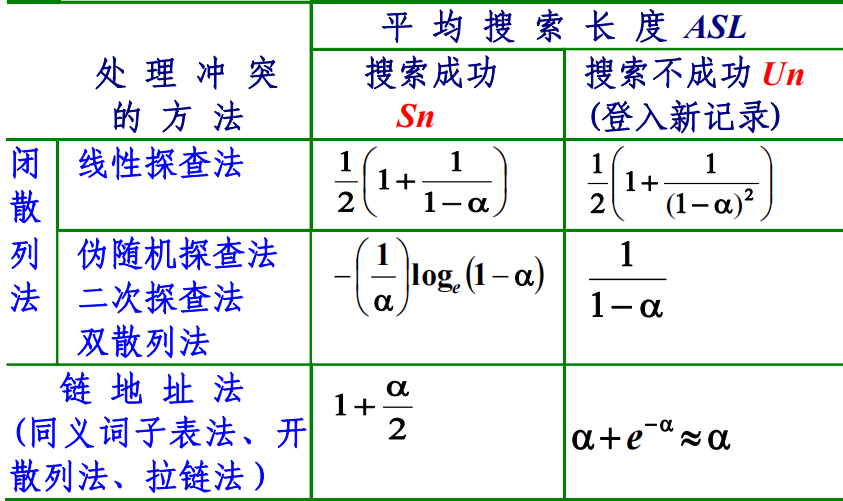
image1)Summary
Comparison between Binary Search Trees and Hash Tables
-
difficult to find the minimum (or maximum) element in a hash table
-
Can not find a range of elements in a hash table
-
$O(\log_2n)$ is not necessarily much more than $O(1)$,since there are no multiplications or divisions by BSTs
-
Sorted input can make BSTs perform poorly